In some cases you will need to enter all your own inputs for CASA tasks. In other cases, inputs are given here. You are encouraged to modify the inputs as ou want anc create your own script.
The input data are calibrated, but in some cases with added errors. In most case a single spectral window has been split out for 3C277.1 (1252+5634) and its phase reference source (1302+5748), averaged to 16 8-MHz channels.
It is best to work in a different directory from the one you used for earlier tutorials to avoid confusing datasets with similar or even the same names. You need less than 1 G. Download and extract the data using
wget -c http://almanas.jb.man.ac.uk/amsr/3C277p1/3C277.1erroranalyse.tar

tar -xvf 3C277.1erroranalyse.tar
You should have:
1302+5748_3.split.ms
1302+574_3.clean.image
1302+5748_ERROR1.split.ms
1302+5748_ERROR1.image
1302+5748_ERROR2.split.ms
1302+5748_ERROR2.image
1302+5748_ERROR3.split.ms
1302+5748_ERROR3.image
1252+5634_statwtOK_3.ms
1252+5634_3OK.clean.image
1252+5634_ERROR4.ms
1252+5634_ERROR4.image
1252+5634_ERROR5.ms
1252+5634_ERROR5.image
1252+5634_ERROR5_big.image
1252+5634_statwt.clean.image.tt0
1252+5634_statwt.clean.image.alpha
1252+5634_statwt.clean.image.alpha.error
Start CASA.
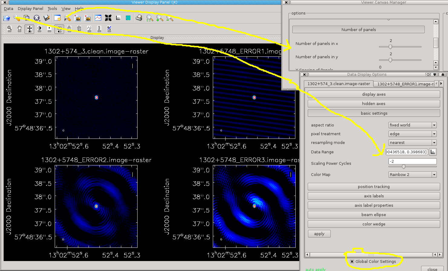
Start the Viewer and make 4 panels. Load as raster images:
1302+574_3.clean.image (the 'good' image)
1302+5748_ERROR1.image
1302+5748_ERROR2.image
1302+5748_ERROR3.image
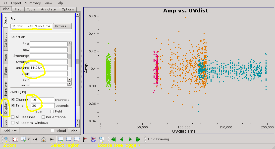
See if you can identify possible causes of error. Then use plotms to look at each parent MS (easier to see if you use 16-channel, 10 sec averaging). Plot amplitude and phase against time or uvdistance. When you spot some bad data you can either use Select and Locate, or colourise (Display tab) or iterate through baselines (Page tab) to identify the timerange or antenna responsible.
Examining the non-error visibilities Note the noisier data around 100,000 m baselines are the less-sensitive De antenna, not an error.
If it is just a couple of bad points you can flag them (interactively or, better, using flagdata). If a long period is mis-scaled (but otherwise coherent, not just noise) for a single antenna, call this A, you can try using an image made from the other antennas as a model to calibrate the data for all antennas:
# In CASA:
A = '!some antenna'               # !  means do not use this antenna
V = 'an error visibility data set'

clean(vis=V,
      imagename='1302+574_3noA.clean',
      cell='0.012arcsec',
      niter=100,
      antenna=A
      mask='circle [[128pix,128pix],5pix ]',
      interactive=T,
      imsize=256)
# In CASA:
GOUT = 'name for gain table'
os.system('rm -rf '+GOUT)
gaincal(vis=V,
        calmode='ap',
        caltable=GOUT,
        solint='180s',
        refant='Mk2',          # change if this is the bad one!
        minblperant=2,minsnr=2)

applycal(vis=V,
         gaintable=GOUT)
Whether you flag or re-calibrate, image again and see if the error has gone.
These are harder to diagnose just from the images. Load 1252+5634_3OK.clean.image and 1252+5634_ERROR4.image into the viewer. Compare the visibilities (hint: easiest to spot if you plot all baselines, amp against time), remove the problem and check by re-imaging.
Now look at 1252+5634_ERROR5.image and compare the visibilities for 1252+5634_ERROR5.ms (hint: here, amp against uvdistance is most revealing). Note that these data have not had the extra channel averaging.
Compare ERROR5 and the original visibilitiesIf you are stuck, look at 1252+5634_ERROR5_big.image and zoom in on the bottom left.
A wider field around ERROR5There are two steps towards getting rid of confusion; firstly to image the field including masking the offending source, which will produce an improvement (compare the noise close to the target in 1252+5634_ERROR5.image and in the larger image 1252+5634_ERROR5_big.image, where the confusion was masked), This may be sufficient, but you can go further and subtract it from the visibility data as well. If you have time, try this recipe below. Cleaning separate fields is quicker than one huge image and is needed for the subtraction.
# In CASA
# Clean the target and the confusion, setting masks
os.system('rm -rf 1252+5634_3?.clean*')
clean(vis='1252+5634_ERROR5.ms',
      imagename=['1252+5634_3a.clean','1252+5634_3b.clean'],
      cell='0.012arcsec',
      niter=2500,
      npercycle='500,
      phasecenter=['J2000 12h52m26.2859 +56d34m19.488','J2000 12h52m28 +56d34m05'],
      interactive=T,
      imsize=[[512,512],[256,256]])
Insert the clean components just for the confusing source into the MS
# In CASA:

ft(vis='1252+5634_ERROR5.ms',
   model='1252+5634_3b.clean.model',
   usescratch=T)
Use plotms to plot the model
Subtract the model from the visibilities
uvsub(vis='1252+5634_ERROR5.ms')
This writes the corrected column, so now compare that in plotms (tick 'reload').
Finally, re-image (using your old masks to save time - but you can hopefully delete the confusion mask!)
# In CASA:

os.system('rm -rf 1252+5634_3sub?.clean*')
clean(vis='1252+5634_ERROR5.ms',
      imagename=['1252+5634_3suba.clean','1252+5634_3subb.clean'],
      cell='0.012arcsec',
      niter=2500,
      npercycle='500,
      phasecenter=['J2000 12h52m26.2859 +56d34m19.488','J2000 12h52m28 +56d34m05'],
      mask=['1252+5634_3a.clean.mask','1252+5634_3b.clean.mask'],
      interactive=T,
      imsize=[[512,512],[256,256]])
Once you have made an image, you can use exportfits to write it out as a FITS file and use any package you like (see talk for caveats and suggestions). These are just a few of the things you can do in CASA. These examples are based on 1252+5634_statwt.clean.image.tt0, 1252+5634_statwt.clean.image.alpha,1252+5634_statwt.clean.image.alpha.error as downloaded but you can use your own best image.
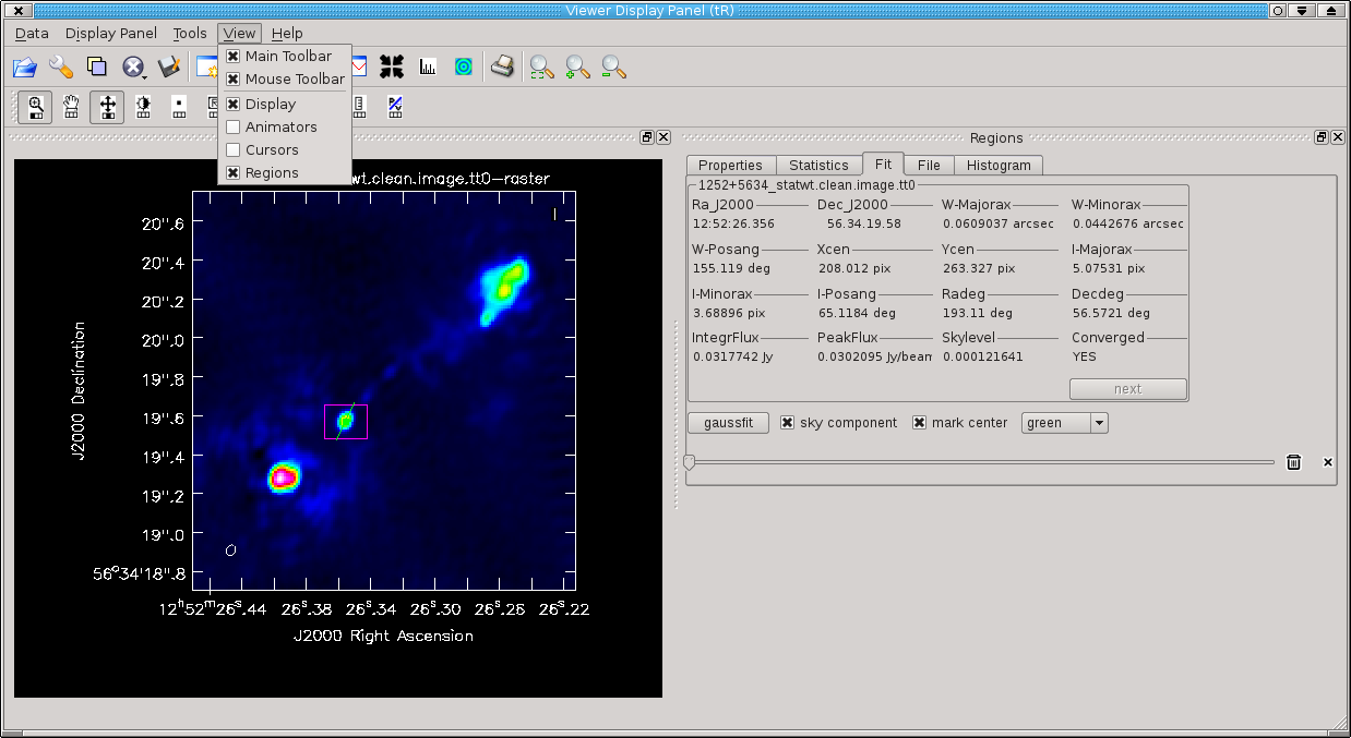
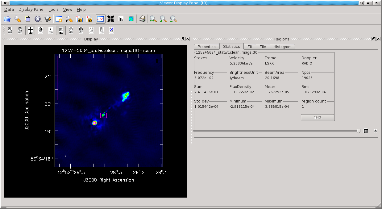
Open 1252+5634_statwt.clean.image.tt0 in the viewer and adjust the color table/zoom in. Open the Regions pane (View menu) and experiment with its options. You can select a peak and fit a Gaussian component, or select an off-source area to measure the noise rms, (Statistics sub-pane) or a histogram of the noise. Cursors (View menu) will let you note the pixel positions of your box corners.
There are also tasks which can be used to measure the noise and other image statistics (imstat) and to fit 2-D Gaussian components (imfit).
To measure the off-source noise, for example:
# In CASA
default imstat
imagename='1252+5634_statwt.clean.image.tt0'
box='10,400,199,499'
imstat
# In CASA
# rms1 and peak1 are variable names you can set to anything allowed by python
# They will take the values of the measured quantities.
rms1=imstat(imagename='1252+5634_statwt.clean.image.tt0',
                  box='10,400,199,499')['rms'][0]
peak1=imstat(imagename=target+'_1.clean.image',
                  box='10,10,499,499')['max'][0]

print  rms %7.3f mJy' % (rms1*1000.)
print  peak %7.3f mJy/bm' % (peak1*1000.)
If you make a clean image with nterms = 2, this fits a spectral index at every pixel. The output images include:
1252+5634_statwt.clean.image.tt0            # Total intensity
1252+5634_statwt.clean.image.alpha          # Spectral index
1252+5634_statwt.clean.image.alpha.error    # Spectral index error
If you inspect 1252+5634_statwt.clean.image.tt0 in the viewer, the noise rms is about 0.08 mJy/bm. -0.7 is a typical spectral index (alpha) for radio galaxies, where
S(nu_2) = S(nu_1) * (nu_2/nu_1)**alpha
(flux density is S(nu_1) at frequency nu_1 etc.)
From listobs previously you can see that the frequency span is about 4.82-5.33 GHz, leading to about 7% decrease in flux density across the band. If we require this difference to be at least 6*rms, this implies 7% of the flux density must be at least 0.5 mJy, or the total flux density must be at least 7 mJy; we use 8 mJy here as a cut-off.
The task immath will blank the spectral index image based on a cut-off level of the total intensity image:
# In CASA

os.system('rm -rf 1252+5634_statwt.clip.alpha*')

default('immath')
imagename=['1252+5634_statwt.clean.image.alpha','1252+5634_statwt.clean.image.tt0']
expr = ' iif( IM1 >=0.008 , IM0, -3) '
outfile = '1252+5634_statwt.clip.alpha'
immath
This means, at each pixel, if the second image is greater than or equal to 0.008 Jy, use the first image, otherwise replace the values in the first image with -3 (a value outside the expected range which will display as black).
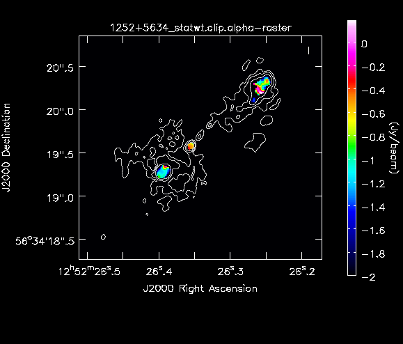
The color shows the spectral index; contours are at (3, 12, 48)x0.08mJy for the total intensity image..
This is roughly consistent with Cotton et al. 2006, i.e. the core has a flatter spectral index than the brighter, E lobe/hotspot. The flat region in the W lobe has lower significance and might be genuine or due to a bad choice of clean mask. You can also overplot the
1252+5634_statwt.clean.image.alpha.error 0.2 or 0.3 contour, showing the area above about 3xerror in spectral index.