This imaging tutorial follows the calibration tutorial in 3C277.1 calibration. Follow the link for details on the data and the source.
You will need to download the associated scripts (and calibrated data set if calibration went badly with your own calibration):
1252+5634.ms.tar - the target 3C277.1 with all external calibration applied
wget -c http://www.jb.man.ac.uk/~radcliff/DARA/Data_reduction_workshops/3C277_eMERLIN/1252+5634.ms.tar
The task names are given below. You need to fill in one or more parameters and values where you see ***. Use the help in CASA, e.g. for clean
taskhelp                        # list all tasks
inp(clean)                      # possible inputs to task
help(clean)                     # help for task
help(par.cell)                  # help for a particular input (only for some parameters)
Extract 1252+5634.ms (NB if you have already tried this tutorial, but want to start from scratch again, you can either use clearcal(vis=1252+5634.ms), or, if you think you have really messed it up, delete it and re-extract the tar file).
tar -xvf 1252+5634.ms.tar
Start CASA, list the contents of the MS (writing the output to a list file for future reference).
# in CASA
listobs(***)
Make a note of the frequency and the number of channels per spw.
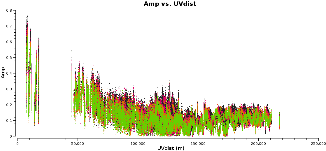
Plot amplitude against uv distance, averaging all channels per spw (just for correlations RR,LL, here and future plotms).
# in CASA
plotms(***)
Note the longest baseline uv distance.
Now, in plotms, using the axes tab, select Data Column model and re-plot. The model should be the default flat1 1 Jy if you have not done any imaging yet.
Work out the imaging parameters.
# in CASA
max_B = ***                        # max. baseline from uv plot (in metres)
wavelength = ***                   # approximate observing wavelength (in metres) - listobs gives the frequency.
theta_B= 3600.*degrees(wavelength/max_B)   # convert from radians to degrees and thence to arcsec
theta_B
To find a good cell size, take theta_B/5 rounded up to the nearest milli-arcsec. To find a good image size, look at Ludke_et_al._1998.pdf page 5, 3C277.1 and estimate the size of that image, in pixels. Due to the sparse uv coverage of e-MERLIN and thus extended sidelobes, the ideal image size is at least twice that in order to help deconvolution. As this is quite a small data set, you can pick a power of two which is larger than that.
# in CASA

os.system('rm -rf 1252+5634_1.clean*')
clean(vis='1252+5634.ms',
      imagename='1252+5634_1.clean',
      cell='**arcsec',                         # The pixel size
      imsize=***,                              # Image size in pixels
      interactive=T)
Set a mask round the obviously brightest regions and clean interactively, mask new regions or increase the mask size as needed. Stop cleaning
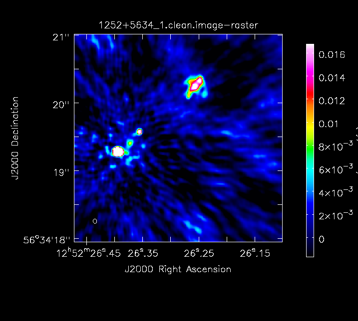
Have a look at the image in the viewer. If you start the viewer and click on an image to load, the synthsised beam is displayed, about 70x50 mas2 for this image.
Measure the noise and peak. This set of boxes are for a 512-pixel image size, change if you used a different size.
# in CASA
rms1=imstat(imagename='1252+5634_1.clean.image',
              box='10,400,199,499')['rms'][0]
peak1=imstat(imagename='1252+5634_1.clean.image',
              box='10,10,499,499')['max'][0]

print '1252+5634_1.clean.image rms %7.3f mJy' % (rms1*1000.)
print '1252+5634_1.clean.image peak %7.3f mJy/bm' % (peak1*1000.)
I got
1252+5634_1.clean.image rms   1.811 mJy
1252+5634_1.clean.image peak 156.438 mJy/bm
This illustrates the use of imview to produce reproducible images; this is optional but shown for reference. You can use the viewer interactively to decide what values to give the parameters. NB If you use the viewer interactively, make sure that the black area is a suitable size to just enclose the image, otherwise imview will produce a strange aspect ratio plot.
# in CASA
imview(raster={'file': '1252+5634_1.clean.image',
               'colormap':'Rainbow 2',
               'scaling': -2,
               'range': [-1.*rms1, 10.*rms1],
               'colorwedge': True},
       zoom=2,
       out='1252+5634_1.clean.png')
 This plot shows the Clean Components (size proportional to amplitude) which you can only overplot directly in the viewer. clean
also puts the Fourier transform of the CC as a model in the measurement
set. Use plotms as in step 1 to plot the model against uv distance.
This plot shows the Clean Components (size proportional to amplitude) which you can only overplot directly in the viewer. clean
also puts the Fourier transform of the CC as a model in the measurement
set. Use plotms as in step 1 to plot the model against uv distance.
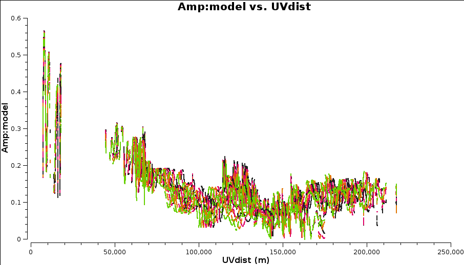
You can also plot data-model which shows that there are still many discrepancies.
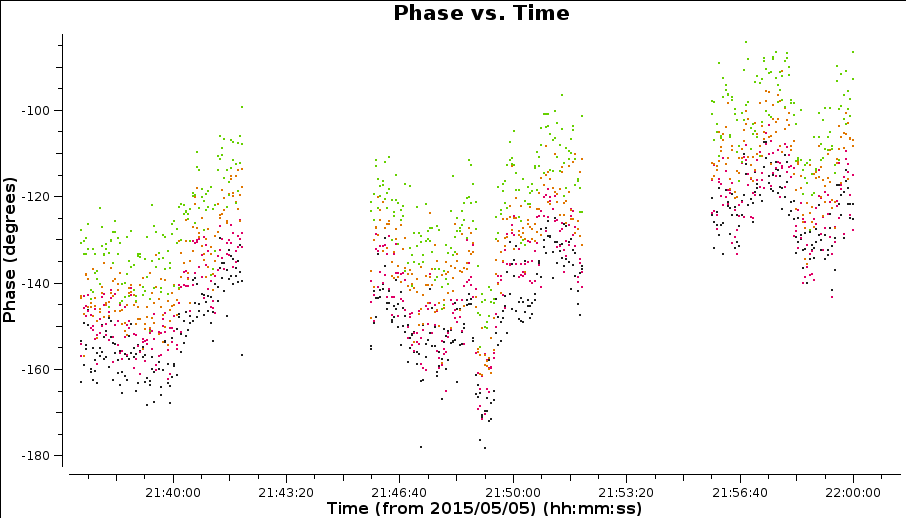
It is hard to tell the difference between phase errors and source structure in the visibilities, but it helps to balance between choosing a longer interval to optimise S/N, and too long an interval (if possible the phase changes by less than a few tens of degrees). The phase will change most slowly due to source structure on the shortest baseline, Mk2&Pi but you should also check that the longest baselines (to Cm) also have enough S/N. Plot phase against time, averaging all channels per spw (see listobs for the number of channels).
# in CASA
plotms(***)
The plot below shows a zoom on a few scans. The chosen solint should also ideally fit an integral number of times into each scan, and it is a good idea not to use too short a solution interval for the first model as it may not be very accurate so you don't want to constrain the solutions too tightly.
Use gaincal to derive solutions
# in CASA
os.system('rm -rf target.p1')
gaincal(vis='***',
        caltable='target.p1',
        field='***',
        solint='***s',                            # about half a scan duration
        calmode='***',                            # phase only
        refant='***',
        minblperant=2,minsnr=2)                   # These are set to lower values than the defaults which are for arrays with many antennas
Check the terminal and logger; there should be no (or almost no) failed solutions.
Plot solutions
# in CASA
plotcal(caltable='target.p1',
        xaxis='time',
        yaxis='phase',
        plotrange=[-1,-1,-180,180],
        iteration='antenna',
        subplot=321,
        poln='L')
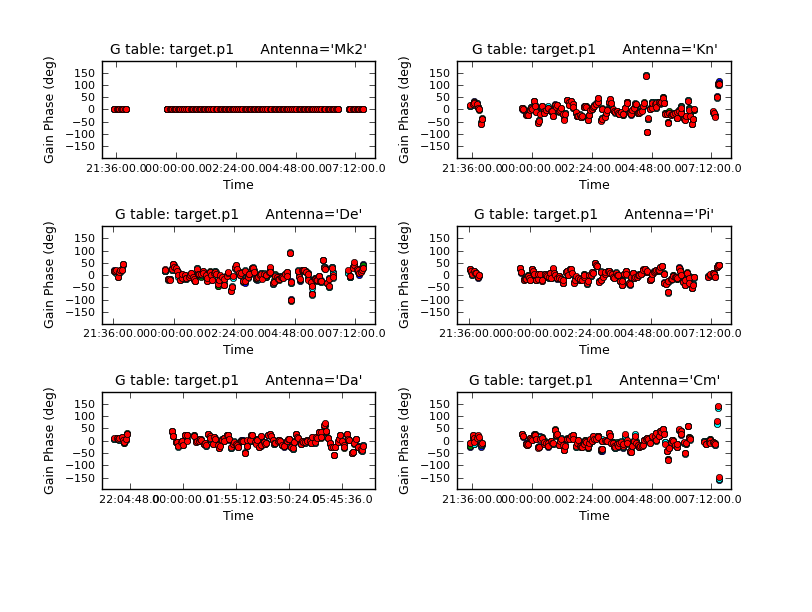
Repeat for the other polarization. The corrections should be coherent, as they are, and represent the difference caused by the different atmospheric paths between the target and phase-ref, but they may also have a spurious component if the model was imperfect. The target is bright enough that a shorter solution interval could be used. So, these solutions are applied, the data re-imaged and the corrections refined iteratively.
== Apply first phase solutions and image again (step 5)==
# in CASA
applycal(***)    # enter the name of the MS and the gaintable
Clean again, as before, but you might be able to do more iterations as the noise should be lower.
# in CASA
os.system('rm -rf 1252+5634_p1.clean*')
clean(vis='***',
      imagename='1252+5634_p1.clean',
      ***)
Use imstat to find the rms again and viewer to inspect the image, and plot it if you want. I got
1252+5634_p1.clean.image rms   0.405 mJy
1252+5634_p1.clean.image peak 164.940 mJy/bm
Check that the S/N has improved.
Now that the model is better, use a shorter solution interval. Heuristics suggest that 30s is usually about the shortest worth using, since the atmosphere is reasonably stable on these baseline lengths at this frequency.
Run gaincal as before, but reduce the solint to 30s and write a new solution table (the new model will be used).
# in CASA
os.system('rm -rf target.p2')
gaincal(vis='***',
        caltable='target.p2'
        ***)
Plot the solutions.
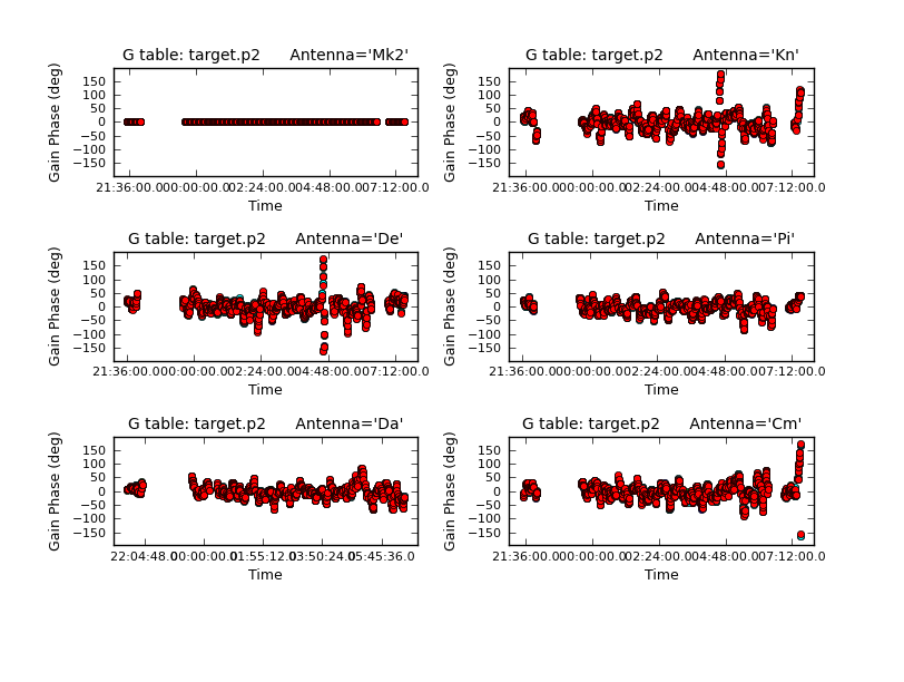
Use applycal as before, just changing the name of the gaintable to the new one.
From listobs, the total bandwidth is almost 10% of the frequency, which is enough to take the spectral index into account. Cotton_et_al._2006 finds a spectral index varies from -0.1 in the core to as steep as -1. Listobs showed the total bandwidth is 4817 to 5329 MHz, i.e. for flux density S, S4817/S5329 = (4817/5329)-1 or about 10%. The improved S/N gives much greater accuracy. Thus, in order to image properly and produce an accurate image to amplitude self-calibrate all spectral windows, MFS (multi-frequency synthesis) imaging is used; this solves for the spectral index across the map.
Make sure you clean till as much target flux as possible hase been removed into the model - you can increase the number of iterations interactively if you want.
# in CASA
os.system('rm -rf 1252+5634_p2.clean*')
    clean(vis='***',
          imagename='1252+5634_p2.clean',
          nterms=2, # Make spectral index image with a linear fit
          ***)
Use ls to see the names of the image files created. The image is 1252+5634_p2.clean.image.tt0
Check the image as before. I got
1252+5634_p2.clean.image.tt0 rms   0.277 mJy
1252+5634_p2.clean.image.tt0 peak 170.216 mJy/bm
Plot amplitude against time in order to choose a suitable solution interval.
# in CASA
plotms(***)
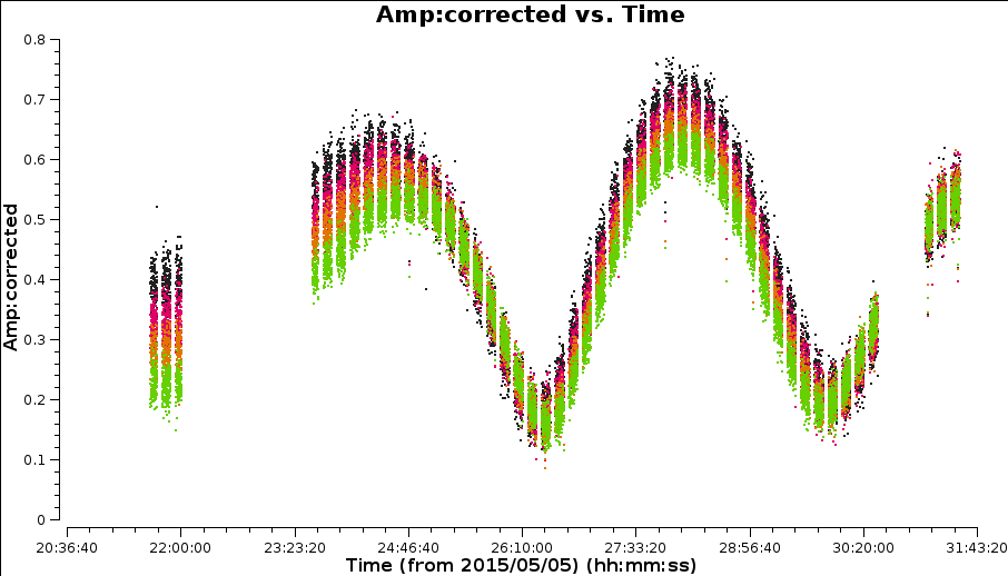
The amplitudes change more slowly than phase errors and a suitable solint is a few times longer than for phase.
In gaincal, the previous gaintable with short-interval phase solutions will be applied, to allow a longer solution (averaging) interval for ampliude self-calibration. Set up gaincal to calibrate amplitude and phase, with a longer solution interval, and the same refant etc. as before.
# in CASA
os.system('rm -rf target.ap1')
gaincal(vis=target+'.ms',
       caltable='target.ap1',
       .....
       gaintable='target.p2',           # this table will be applied
       minblperant=2,minsnr=2)
Plot the solutions. They should mostly be within about 20% of unity. A few very low points implies some bad data (high points); if the solutions are consistently much greater than unity then the model is missing flux.
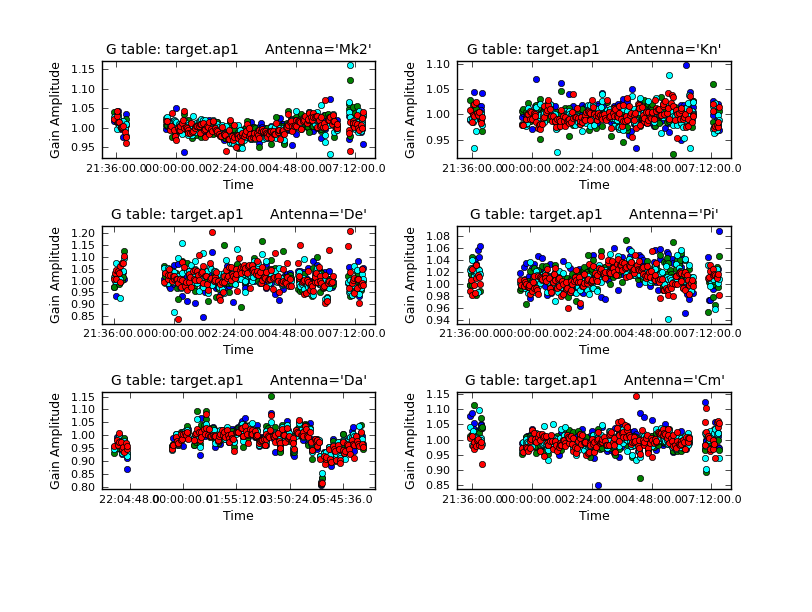
Use applycal to apply the short-interval phase solution table and the amplitude and phase table you have just created.
clean the image again, as before and inspect. I got:
1252+5634_ap1.clean.image.tt0 rms   0.138 mJy
1252+5634_ap1.clean.image.tt0 peak 170.162 mJy/bm
The noise should have gone down, but the peak should not have changed significantly.
You can select weight for the y-axis in plotms. However, e-MERLIN weights are not handled correctly by all versions of CASA so we can try re-calculating them, based on the scatter in small samples of data. The original data are overwritten so you might want to copy the MS to a different name or directory first.
# in CASA
statwt(vis='***')                   # all default apart from input data set
Plot again in plotms. The Cm antenna is larger and more sensitive, which shows!
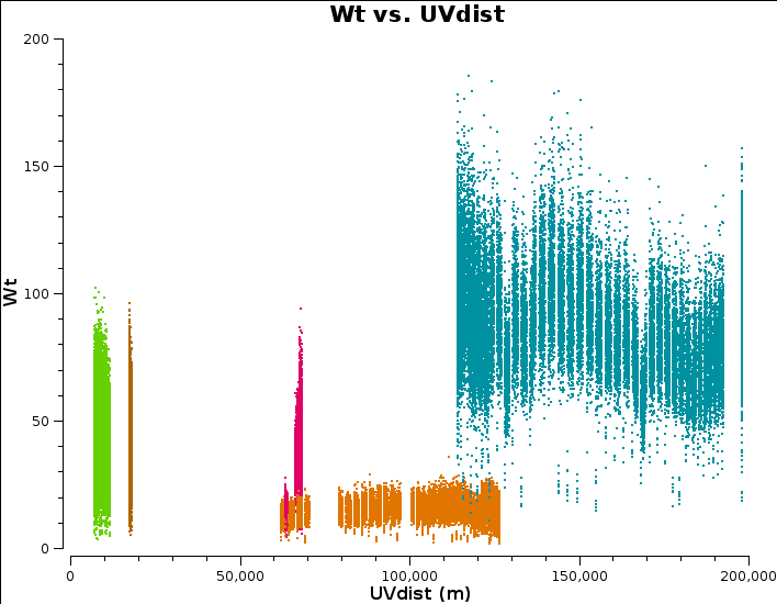
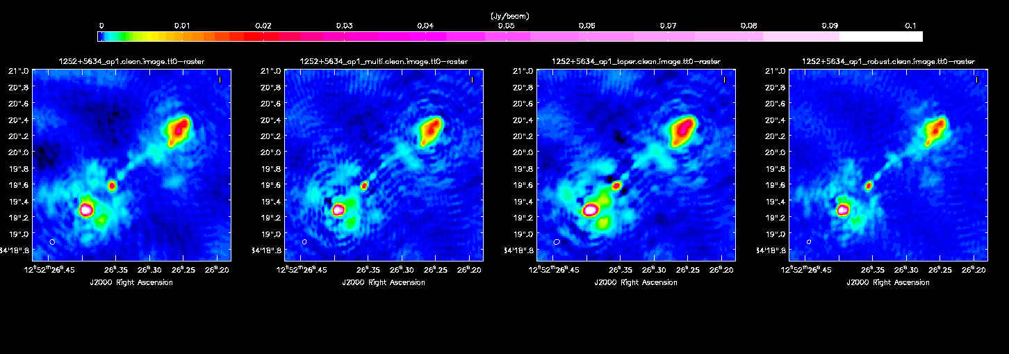
Image the re-weighted data using multiscale clean, which looks for groups of Clean Components instead of treating each independently. Have a look at the help for clean, which suggests suitable values of the multiscale parameter.
# in CASA
os.system('rm -rf 1252+5634_ap1_multi.clean*')
clean(vis='1252+5634.ms',
      imagename='1252+5634_ap1_multi.clean',
      ...
      multiscale=[**,**,**],
      ***}
You will find that the beam is now slightly smaller (I got 60x40 mas2) as the longer baselines have more weight, so the peak is lower. I got
1252+5634__ap1_multi.clean.image.tt0 rms   0.086 mJy
1252+5634__ap1_multi.clean.image.tt0 peak 148.394 mJy/bm
Experiment with changing the relative weights given to longer baselines. Applying a taper reduces this, giving a larger synthesised beam more sensitive to extended emission. This just changes the weights during gridding for imaging, no permanent change to the uv data. However, strong tapering increases the noise.
Look at the uv distance plot and choose an outertaper (half-power of Gaussian taper applied to data) which is about 2/3 of the longest baseline. Units are wavelengths, so calculate that or plot amp v. uvwave
# in CASA
os.system('rm -rf 1252+5634_ap1_taper.clean*')
clean(vis=1252+5634.ms',
      imagename='1252+5634_ap1_taper.clean',
      ...
      multiscale=[**,**,**],
      uvtaper=T,
      outertaper='***',
      ***}
Inspect the image and check the beam size. I got 70x60 mas2 and
1252+5634_ap1_taper.clean.image.tt0 rms   0.109 mJy
1252+5634_ap1_taper.clean.image.tt0 peak 183.112 mJy/bm
Experiment with changing the relative weights given to longer baselines. Default natural weighting gives zero weight to parts of the uv plane with no samples. Briggs weighting interpolates between samples, giving more weight to the interpolated areas for lower values of robust. For an array like e-MERLIN with sparser sampling on long baselines, this has the effect of increasing their contribution, i.e. making the synthesised beam smaller. This may bring up the jet/core, at the expense of the extended lobes. Low values of robust increase the noise. You can combine with tapering or multiscale, but initially remove these parameters.
# in CASA
os.system('rm -rf 1252+5634_ap1_robust.clean*')
clean(vis=1252+5634.ms',
      imagename='1252+5634_ap1_robust.clean',
      ...
      weighting='briggs',
      robust=***,                     # choose a value less than 2 and greater than 0
      ***}
I got a beam of 50x40 mas and
1252+5634_ap1_robust.clean.image.tt0 rms   0.065 mJy
1252+5634_ap1_robust.clean.image.tt0 peak 146.100 mJy/bm
Finally, experiment for yourself. You might also find a little more bad data to flag, or even do more calibration if you have a better model.
Script with all commands to follow the tutorial: 3C277.1_imaging.py