This guide provides a basic example for calibrating e-MERLIN C-Band (5 GHz) continuum data in CASA. It has been tested in CASA 4.3-5.3. It is designed to run using an averaged data set all_avg.ms (1.7 G), in which case you will need at least 5.5 G disk space to complete this tutorial.
If you have a very slow laptop, you are advised to skip some of the plotms steps (see the plots linked to this page instead) and especially, do not use the plotms options to write out a png. This is not used in this web page, but if you run the script as provided, you are advised to comment out the calls to plotms or at least the part which writes a png, see tutors for guidance.
3C277.1 is a twin-lobed radio galaxy. These C-band (4-7.3 GHz) e-MERLIN observations were made specifically for this tutorial but previous MERLIN and VLA images have been published by Ludke et al. 1998 and Cotton et al. 2006 . The e-MERLIN User Support web page describes e-MERLIN data in more detail, including the Cookbook and the AIPS pipeline
The CASA home pages describe downloading and installing CASA; also see Getting Started in CASA .
Data all_avg.ms.tar ( wget -c http://almanas.jb.man.ac.uk/amsr/3C277p1/all_avg.ms.tar ) 1.6 GB
Script equivalent of this guide, to be filled: 3C277.1_cal_outline.py
Amplitude calibrator model ( wget -c http://almanas.jb.man.ac.uk/amsr/3C277p1/3C286_C.clean.model.tt0.tar )
tar xvf all_avg.ms.tar
tar xvf 3C286_C.clean.model.tt0.tar
You should be working in the directory containing the data all_avg.ms, the script 3C277.1_cal_outline.py, and 3C286_C.clean.model.tt0
This User Guide presents inputs for CASA tasks e.g. gaincal to be entered interactively at a terminal prompt for the calibration of the averaged data and initial target imaging. This is useful to examine your options and see how to check for syntax errors. You can run the task directly by typing gaincal at the prompt; if you want to change parameters and run again, if the task has written a calibration table, delete it (make sure you get the right one) before re-running. You can review these by typing:
# In CASA:
!more gaincal.last
taskname           = "gaincal"
vis                =  "all_avg.ms"
caltable           =  "bpcals_precal.ap1"
...
...

#gaincal(vis="all_avg.ms",caltable="bpcals_precal.ap1",field="1407+284",spw="",intent="",
selectdata=True,timerange="",uvrange="",antenna="",scan="",observation="",msselect="",solint="120s",
combine="",preavg=-1.0,refant="Mk2",minblperant=2,minsnr=2,solnorm=True,gaintype="G",smodel=[],
calmode="ap",append=True,splinetime=3600.0,npointaver=3,phasewrap=180.0,docallib=False,callib="",
gaintable=['all_avg.K', 'bpcals_precal.p1'],gainfield=[''],interp=[],spwmap=[],parang=False)
When you are happy with the values which you have set for each parameter, enter them in the script 3C277.1_cal_outline.py (or whatever you have called it). You can leave out parameters for which you have not set values; the defaults will work for these (see e.g. help(gaincal) for what these are), but feel free to experiment if time allows.
The script already contains most plotting inputs in order to save time. Make and inspect the plots; change the inputs if you want, zoom in etc. There are links to copies of the plots (or parts of plots) but only click on them once you have tried yourself or if you are stuck.
The parameters which should be set explicitly or which need explanation are given below, with ** if they need values.
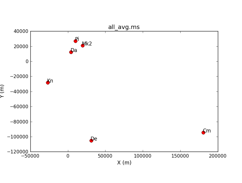
If you have already plotted the antenna positions with plotants you will have seen that Mk2 has many short baselines which makes it more likely to give good calibration solutions and it makes a good reference antenna (refant).
The imput data set all_avg.ms contains five fields:
| e-MERLIN name | Common name | Role |
|---|---|---|
| 1252+5634 | 3C277.1 | target |
| 1302+5748 | J1302+5748 | phase reference source |
| 1407+284 | OQ208 | bandpass cal. (usually about 2 Jy at 5-6 GHz) |
| 0319+415 | 3C84 | bandpass, polarization leakage cal. (usually 10-20 Jy at 5-6 GHz) |
| 1331+305 | 3C286 | flux, polarization angle cal. (flux density known accurately, see Step 7) |
These data were taken in full polarization in 0.512 GHz bandwidth centred on 5072 MHz, in 4 adjacent spectral windows (spw's, also known as IFs). Each 128-MHz spw contains 512 channels 0.25 MHz wide and 1 s integrations were used (the data are later averaged).
The preprocessing of the original raw fits idi files involved (see the full script e-MERLIN-CASA_v0.1.py steps 1-3 for details):
Check that you have all_avg.ms in a directory with enough space and start CASA.
Enter the parameter to specify the MS and, optionally, the parameter to write the listing to a text file.
# in CASA
listobs(***)
Because e-MERLIN stores data for each source in a separate fitsidi file, the sources are listed one by one even though the phase-ref and target scans interleave. So selected entries from listobs, re-ordered by time, show:
Timerange (UTC)          Scan  FldId FieldName             nRows
  SpwIds   Average Interval(s)  #(i.e. RR RL LR LL integration time) 05-May-2015
...
20:02:08.0 - 20:05:08.5     7      0 1302+5748                 2760  [0,1,2,3]  [3.91, 3.91, 3.91, 3.91]    # phase-ref
20:05:11.0 - 20:12:33.5    72      1 1252+5634                 6660  [0,1,2,3]  [3.98, 3.98, 3.98, 3.98]    # target
20:12:36.0 - 20:15:34.5     8      0 1302+5748                 2700  [0,1,2,3]  [3.96, 3.96, 3.96, 3.96]    # phase-ref
...
22:02:04.0 - 22:47:00.5   132      2 1331+305                 40500  [0, 1, 2, 3]  [3.99, 3.99, 3.99, 3.99] # flux scale/pol angle calibrator
22:47:03.0 - 23:29:59.5   133      3 1407+284                 38700  [0, 1, 2, 3]  [3.99, 3.99, 3.99, 3.99] # bandpass calibrator
06-May-2015
07:30:03.0 - 08:29:59.5   134      4 0319+415                 54000  [0, 1, 2, 3]  [4, 4, 4, 4]             # bandpass/leakage calibrator
There are 4 spw
  SpwID  Name   #Chans   Frame   Ch0(MHz)  ChanWid(kHz)  TotBW(kHz) CtrFreq(MHz)  Corrs
  0      none      64   TOPO    4817.000      2000.000    128000.0   4880.0000   RR  RL  LR  LL
  1      none      64   TOPO    4945.000      2000.000    128000.0   5008.0000   RR  RL  LR  LL
  2      none      64   TOPO    5073.000      2000.000    128000.0   5136.0000   RR  RL  LR  LL
  3      none      64   TOPO    5201.000      2000.000    128000.0   5264.0000   RR  RL  LR  LL
and 6 antennas
ID   Name  Station       Diam.    Long.         Lat.                 ITRF Geocentric coordinates (m)
  0    Mk2   e-MERLIN:02 24.0 m   -002.18.08.9  +53.02.58.7     3822473.365000  -153692.318000  5085851.303000
  1    Kn    e-MERLIN:05 25.0 m   -002.59.44.9  +52.36.18.4     3859711.503000  -201995.077000  5056134.251000
  2    De    e-MERLIN:06 25.0 m   -002.08.35.0  +51.54.50.9     3923069.171000  -146804.368000  5009320.528000
  3    Pi    e-MERLIN:07 25.0 m   -002.26.38.3  +53.06.16.2     3817176.561000  -162921.179000  5089462.057000
  4    Da    e-MERLIN:08 25.0 m   -002.32.03.3  +52.58.18.5     3828714.513000  -169458.995000  5080647.749000
  5    Cm    e-MERLIN:09 32.0 m   +000.02.19.5  +51.58.50.2     3919982.752000     2651.982000  5013849.826000
Click here to see the output you would have got for the listing of all_avg.ms: all_avg.listobs.txt
Enter one parameter to plot the antenna positions (optionally, a second to write this to a png).
# in CASA
plotants(***)
Consider what would make a good reference antenna. Although Cambridge has the largest diameter, it has no short baselines.
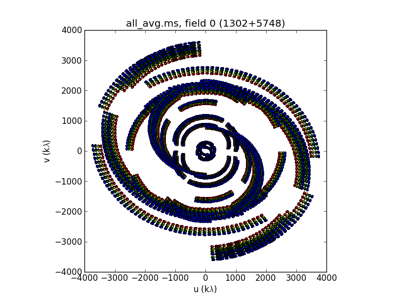
Plot the uv coverage of the data for the phase-reference source. See annotated listobs output above to identify this. You need to enter several parameters; some have been done for you:
# in CASA
plotuv(vis='***',
       field='***',                # phase-ref
       maxnpts=10000000,           # to plot all the data
       symbol='.',                 # a dot which will have a different colour for each spw
       figfile='')                 # fill this in if you want a png
The u and v coordinates represent (wavelength/projected baseline) as the Earth rotates whilst the source is observed. Thus, as each spw is at a different wavelength, it samples a different part of the uv plane, improving the aperture coverage of the source, allowing Multi-Frequency Synthesis (MFS) of continuum sources.
Use plotms to plot the phase-reference source amplitudes as a function of time. Just a few central channels are selected and averaged; enough to give good S/N but not so many that phase errors across the band cause decorrelation (in real life, you might have to experiment with different selections or plot phase v. channel to make the selection).
# in CASA
plotms(vis='***',
       field='***',         # phase-ref
       spw='0~3:20~43',     # plot just the inner 3/8 of the channels for each spw (see listobs output)
       avgchannel='***',    # average these channels
       xaxis='**',
       yaxis='**',
       antenna='Mk2&*',     # This uses Mk2 as refant for ease of comparision but another with many short baselines could be used.
       correlation='**,**', # Just select the parallel hands, since the cross hands (polarised intensity) are much fainter.
       coloraxis='***')     # Color by baseline or correlation as you prefer
You can change the parameters interactively once plotms has started.
Roughly the same interval at the start of each scan is bad for all sources and antennas, so the phase reference is a good source to examine. (In a few cases there is extra bad data, ignor that for now). Use zoom, and Tools hover and display to estimate the time interval and enter it in flagdata as below.
First, back up the existing flagging state
# in CASA
flagmanager(***)       # Set the input file name, the mode to save the existing flagging state, and a name to save in.
Use flagdata mode quack to flag the first few tens of seconds (as you identified from plotms) of each scan.
# in CASA
flagdata(vis='***',
         mode='***',
         quackinterval=***)
Re-plot in plotms (tick reload option and replot if you
still have it open) to check that the bad data at the start of each scan
are gone. There are still some irregular periods of bad data which
will be flagged later. 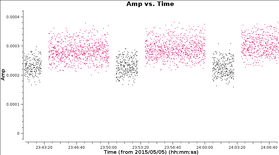
The edges of the bandpass for each spw are low sensitivity and must be flagged. This is the same for all sources, polarizations and antennas but different spectral windows may be different. Just look at the brightest source, 0319+415.
# in CASA
plotms(vis='***',
       field='***',
       xaxis='***',yaxis='***',                          # plot amplitude against channel
       antenna='***',                                    # select one baseline
       correlation='**,**',                                # just parallel hands
       avgtime='***',                                    # set to a large number
       avgscan=*,                                        # average all scans
       iteraxis='***',                                   # view each spectral window in turn
       coloraxis='***')                                  # as you please
Note the channel ranges which are significantly less sensitive at each end of each spw.
Back up the flags and enter the appropriate parameters in flagdata
# in CASA

flagmanager(***)

flagdata(vis='***',
         mode='manual',
         spw='0:0~6;60~63,***')   # enter the ranges to be flagged for the other spw
Re-plot in plotms
Finally, you usually have to go through all baselines, averaging channels and plotting amplitude against time. To save time (and sanity!), you don't have to do it all here. Have a look at 0319+419 and write down a few commands. This is done in the form of a list file, which has no commas and the only spaces must be a single space between each parameter for a given flagging command line. Some errors affect all the baselines to a given antenna; others (e.g. correlator problems) may only affect one baseline. Usually all spw will be affected so you can just inspect one but check afterwards that all are 'clean'. It can be hard to see what is good or bad for a faint target but if the phase-ref is bad for longer than a single scan then usually the target will be bad for the intervening time. Because the data are taken over two days,it is safest to use the full date for any timerange.
Back up the flags with flagmanager
Use plotms to inspect 0319+415, plotting amplitude against time, RR,LL only, averaging all channels, all baselines to Mk2, paging (iterating) through the baselines.
Here are the flagging commands in list format for the data shown below
mode='manual' field='0319+415' timerange='2015/05/06/07:30:00~07:35:00'
mode='manual' field='0319+415' antenna='Da' timerange='2015/05/06/07:30:00~07:56:22'
mode='manual' field='0319+415' antenna='Mk2&Kn' timerange='2015/05/06/07:30:00~07:35:34'
mode='manual' field='0319+415' antenna='Mk2&Kn' timerange='2015/05/06/07:48:55~07:48:58'
mode='manual' field='0319+415' antenna='Mk2,De' timerange='2015/05/06/07:35:00~07:35:18'
mode='manual' field='0319+415' timerange='2015/05/06/08:28:30~08:30:00'
Note that, by paging through all the baselines, you can figure out what bad data affect which antennas.
Have a look at 1331+305 and write its commands.
The commands are applied in flagdata using mode='list', inpfile='***' where inpfile is the name of the flagging file. Write a file all_avg_1.flags with all the commands to flag bad data. Apply it in flagdata using mode 'list'. Look carefully at the messages in the logger and terminal in case any syntax errors are reported.
Re-plot the data to check that it is now clean!
Plot the raw phase against frequency for a bright source. This is usually a bandpass calibrator.
#In CASA:
 default plotms
 vis='all_avg.ms'
 field='0319+415'
 xaxis='frequency'
 gridrows=5;gridcols=1;iteraxis='baseline'    # Plot multiple baselines on one page
 yaxis='phase'
 antenna='Mk2&*'                              # Plot all baselines to the reference antenna
 avgtime='600'                                # Average 10 min
 correlation='LL,RR'
 coloraxis='corr'

# Type plotms to start the plotter
# You can change parameters interactively in plotms
The y-axis spans -200 to +200 deg and some data has a slope of about a full 360 deg across the 512-MHz bandwidth.
QUESTION 1 What is the apparent delay error this corresponds to? What will be the effect on the amplitudes? Answer 1
QUESTION 2 Delay corrections are calculated relative to a reference antenna which has its phase assumed to be zero, so the corrections factorised per other antenna include any correction due to the refant. Roughly what do you expect the magnitude of the Cm corrections to be? Do you expect the two hands of polarization to have the same sign? Answer 2
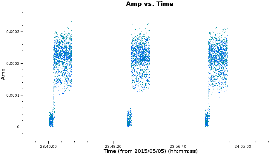
Plot amplitude against time for just one channel per spw.
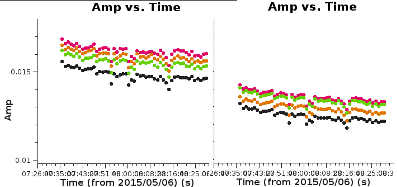
# In CASA:
 default plotms
 vis='all_avg.ms';field='0319+415'
 avgtime='60';antenna='Mk2&Cm';correlation='RR'     # 60-sec average, one baseline/pol
 xaxis='time';yaxis='amp';ydatacolumn='data'        # Plot amplitude v. time with fixed y scale
 plotrange=[-1,-1,0.01,0.018];coloraxis='spw'
 spw='0~3:55'                                       # Just one channel per spw
 plotms
# In CASA:
 default plotms
 vis='all_avg.ms';field='0319+415'
 avgtime='60';antenna='Mk2&Cm';correlation='RR' # 60-sec average, one baseline/pol
 xaxis='time';yaxis='amp';ydatacolumn='data'        # Plot amplitude v. time with fixed y scale
 plotrange=[-1,-1,0.01,0.018];coloraxis='spw'
 spw='0~3';avgchannel='64'                          # Average all unflagged channels
 plotms
Plots of amplitudes for 3C84, Mk2-Cm, pol RR for a single channel (left) and all channels (right).
QUESTION 3 In the plots, which has the higher amplitudes - the channel-averaged data or the single channel? Why? Answer 3
The CASA task gaincal is used to derive most calibration. Type inp gaincal or help gaincal to find out more. Fill in the **.
# In CASA:
 os.system('rm -rf all_avg.K')                   # Remove any old version
 default gaincal
 vis='all_avg.ms'
 gaintype='**'                                   # Delay calibration (see help gaincal)
 field= '1302+5748,0319+415,1407+284,1331+305'   # All calibration sources
 caltable='all_avg.K'                            # Output table containing corrections
 spw='0~3'
 solint='**'                                     # 600s solution interval
 refant='**'                                     # Reference antenna (phase set to origin)
 minblperant=2                                   # For each antenna and solint, require solutions on
 minsnr=2                                        # at least 2 baselines with S/N > 2

 inp gaincal                                     # check inputs

**                                               # Type the task name to run
Inspect the solutions. Are they of the magnitude you expect?
# In CASA:
 default plotcal
 caltable='all_avg.K'
 xaxis='**';yaxis='**'                  # Plot delay against time
 subplot=321; iteration='antenna'       # Each antenna in a separate pane, coloured by spw
 figfile='all_avg.K.png'
The solutions are stable in time, showing that the phase ref solutions can be applied to the target.
1331+305 (= 3C286) is an almost non-variable radio galaxy and its total flux density is very well known as a function of time and frequency (Perley & Butler 2013) . It is somewhat resolved by e-MERLIN, so we use a model made from a ~12-hr observation centred on 5.5 GHz. This is scaled to the current observing frequency range (around 5 GHz) using {{setjy}} which derives the appropriate total flux density, spectral index and curvature using parameters from Perley & Butler (2013). However, a few percent of the flux is resolved-out by e-MERLIN; the simplest way (at present) to account for this is later to scale the fluxes derived for the other calibration sources by 0.938 (based on calculations for e-MERLIN by Fenech et al.).
The model is a set of clean components (see Imaging tutorial) and setjy enters these in the Measurement Set so that their Fourier transform can be used as a uv-plane model to compare later with the actual visibility amplitudes. If you make a mistake (e.g. set a model for the wrong source) use task delmod> to remove it.
# In CASA:
 default setjy
 vis='**'
 field='**'
 standard='Perley-Butler 2013'
 model='3C286_C.clean.model.tt0'  # You should have downloaded and untar'd this model
**
By default, setjy scales the model for each channel, as seen if you plot the model amplitudes against uv distance, coloured by spectral window. If you have plotms running, go to the axes and select the model, or see the script for inputs. The model only appears for the baselines present for the short time interval for which 1331+305 was observed here.
Fourier plane model of 1331+305, amp v. uv distanceWe have a Catch 22 situation: in order to derive good time-dependent corrections we need to average amplitude as well as phase in frequency, but in order to average in frequency we need the phase to be flat in time and the amplitude to have the correct spectral index. So we derive initial time-dependent solutions for the bandpass calibration sources, but discard these after they have been applied to derive the initial bandpass solutions. These, in turn, are replaced in script step 11.
Estimate the time-averaging interval for phase by plotting phase against time for a single channel near the centre of the band for a bandpass calibration source. If the results for the first channel you try look bad, it may be a partly flagged channel; try a different one.
# In CASA:
 default plotms
 vis='all_avg.ms'
 field='**'               # Plot bandpass calibrator
 spw='0~3:55'             # This gives all spw, channel 55 in each.
 antenna='**'             # Plot the longest baseline to the refant, likely to have the fastest-changing phase
 xaxis='time'; yaxis='phase';ydatacolumn='data' # Plot raw phase against time, no averaging
 coloraxis='spw'

 **
Zoom to help decide what phase solution interval to use. The integration-to-integration scatter is noise (mostly instrumental) which cannot be removed but the longer-term wiggles are mainly due to the atmosphere and we want to derive corrections to reduce these to about the level of the noise or at least to less than 5-10 deg. The longer a solution interval, the better the S/N but the interval has to be short enough not to average over the wiggles.
Zoom in on plot of 0319+415 uncorrected phase v. time (correlation 'RR')QUESTION 4 The plot shows 4 spw. What other effect, apart from atmospheric phase errors, will be solved by calibrating phase against a point model at the phase centre? Answer 4
# In CASA:
 os.system('rm -rf bpcals_precal.p1')
 default gaincal
 vis='all_avg.ms'
 caltable='bpcals_precal.p1'    # The output solution table
 calmode='**'                   # Solve for phase only as function of time
 field='**, **'                 # Two sources suitable for bandpass calibration were observed
 solint='**'                    # Enter a suitable solution interval
 refant='**'
 minblperant=2; minsnr=2
 gaintable='all_avg.K'          # Apply the delay solutions to allow averaging phase across the band
**
Check the solutions. Each spw should have a coherent set of solutions, not just noise.
# In CASA:
 default plotcal
 caltable='bpcals_precal.p1'
 xaxis='**'; yaxis='**'
 subplot=321;
 plotrange=[-1,-1,-180,180];
 iteration='antenna'
 plotcal
The plot of amplitude against time in Step 6 also showed that the uncorrected amplitudes have only a slow systematic slope with time, so a longer solution interval can be used, minimising phase noise.
QUESTION 5 Why solve for phase separately before solving for amplitude? Answer 5
Now derive amplitude solutions. We have not yet derived flux densities for the bandpass calibration sources so we have to normalise the gains (i.e. individual solutions differ but the product is unity so that the overall flux scale is not affected). Thus we have to derive the solutions separately for each of the two bandpass calibrators but write them to the same solution table.
# In CASA
 os.system('rm -rf bpcals_precal.ap1')
 default gaincal
 vis='all_avg.ms'
 calmode='**'                    # Solve for amplitude and phase v. time
 field='0319+415'
 caltable='bpcals_precal.ap1'    # Output solution table
 solint='**'                     # Longer solution interval
 solnorm=**                      # Normalise the amplitude solutions,
 refant='Mk2'
 minblperant=2;minsnr=2
 gaintable=['all_avg.K','bpcals_precal.p1'] # Apply the existing delay and phase solutions
**
 field='1407+284'
 append=T                        # Add solutions to existing table
**
# In CASA
 default plotcal
 **
Use bandpass to derive solutions for phase and amplitude as a function of frequency (i.e., per channel). In order to allow averaging in time, apply the time-dependent corrections which you have just derived.
# In CASA:
 os.system('rm -rf bpcal.B1')
 default bandpass
 vis='all_avg.ms'
 caltable='bpcal.B1'           # New table with bandpass solutions
 field='**,**'                 # Bandpass calibration sources
 fillgaps=16                   # Interpolate over flagged channels
 solint='inf';combine='scan'   # Average the whole time for each source
 refant='**'
 solnorm=**                    # Normalise solutions
 gaintable=['all_avg.K','bpcals_precal.p1','bpcals_precal.ap1'] # Apply all the tables derived for these sources
 minblperant=2;    minsnr=3
**
You may see messages about failed solutions but these should all be for the end channels which were flagged anyway.
Inspect the solutions in plotcal. The phase corrections are small as the delay solutions were already applied. The amplitude solutions will remove local deviations from the bandpass but the corrections so far assume that the source flux density is flat in each spw.
# In CASA
 default plotcal
 caltable='bpcal.B1'
 xaxis='freq';yaxis='phase';plotrange=[-1,-1,-180,180] # Plot phase solutions v. frequency
 iteration='antenna';subplot=321
 plotcal

 yaxis='amp';plotrange=[-1,-1,-1,-1]       # Plot amp solutions, self-scaled
 plotcal
Apply the delay and bandpass solutions to the calibration sources as a test, to check that they have the desired effect of producing a flat bandpass for the phase-reference. There is no need to apply the time-dependent calibration as we have not derived this for the phase-reference source anyway. Some notes about applycal:
help applycal).The delay correction ('K') table contains entries for all sources except the target. The phase reference scans bracket the target scans so it is OK to use the default 'linear' interpolation.
The bandpass ('B1') table is derived from just two bandpass calibration observation and there may be data for other sources outside these times, so extrapolation in time is needed, using 'nearest'. 'linear' interpolation is OK for the bandpass calibrator in frequency.
If you are finding your laptop is slow, you can skip this applycal and the plotms immediately after and just look at the figures here and go to Step 9.
# In CASA:
 default applycal
 vis='all_avg.ms'
 field='0319+415,1302+5748,1331+305,1407+284'
 calwt=F; applymode='calonly'          # Test, so don't change the weights or flag data with failed solutions
 gaintable=['**','**']                 # Enter the names of the tables used to calibrate the bandpass
 interp=['**,**','**,**'])             # The values depend on which table you listed first.
**
Check that the bandpass corrections are good for all data by plotting the 'before and after' phase reference phase and amplitude against frequency.
# In CASA:
 default plotms
 vis='all_avg.ms'; field='1302+5748'                 # Phase reference
 xaxis='frequency';yaxis='phase';ydatacolumn='data'  # First, plot uncorrected phase
 gridrows=5;gridcols=1;avgtime='600';coloraxis='scan'
 iteraxis='baseline';antenna='Mk2&*';correlation='LL,RR'
 plotms

 ydatacolumn='corrected'                              # Repeat for corrected phase
 plotms

 yaxis='amp';ydatacolumn='data'                       # Uncorrected amplitude
 plotms

 ydatacolumn='corrected'                              # Repeat for corrected amp
 plotms
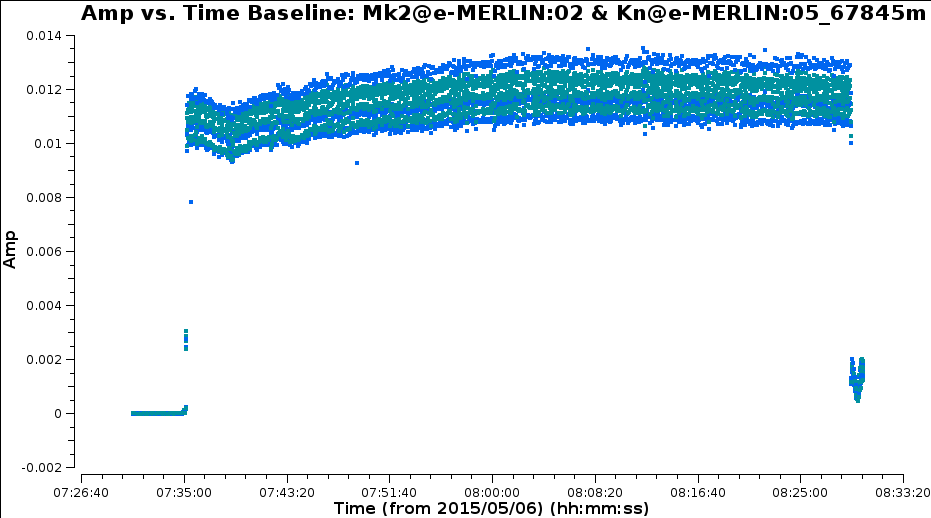
In the Figure, each scan is coloured separately and shows a random offset in phase and some discrepancies in amplitude compared to other scans, but for each individual time interval it is quite flat. So we can average in frequency across each spw and plot the data to show remaining, time-dependent errors.
Plot the corrected phase against time with all channels averaged for the phase reference source. Zoom in on a few scans to deduce a suitable averaging timescale for correction of phase errors as a function of time, i.e. where atmospheric fluctuations dominate over noise.
# In CASA:
 default plotms
 vis='all_avg.ms'; field='1302+5748'
 xaxis='time';yaxis='phase';ydatacolumn='corrected'
 antenna='Mk2&*';iteraxis='baseline'
 avgchannel='64'; coloraxis='spw'
 correlation='LL'    # Just one pol as previous plots show both are similar
 plotms
Repeat for amplitude.
Two scans on the phase ref showing bandpass-corrected amp, coloured by spwDerive time-dependent solutions for all the calibration sources, applying the delay and bandpass tables.
# In CASA:
 os.system('rm -rf calsources.p1')
 default gaincal
 vis='all_avg.ms'
 calmode='p'                           # Phase only first
 caltable='calsources.p1'
 field='**'                            # All calibration sources
 solint='**'                           # Insert solution interval
 refant='Mk2'
 minblperant=2;minsnr=2
 gaintable=['all_avg.K','bpcal.B1']    # Existing correction tables to apply
 interp=['**,**','**,**']              # Insert suitable interpolation modes
 gaincal
When you run gaincal, check the messages in the logger and the terminal.
The logger shows something like:
2015-05-21 06:28:39 INFO gaincal    Calibration solve statistics per spw:
                                             (expected/attempted/succeeded):
2015-05-21 06:28:39 INFO gaincal      Spw 0: 1400/935/930
2015-05-21 06:28:39 INFO gaincal      Spw 1: 1400/935/930
2015-05-21 06:28:39 INFO gaincal      Spw 2: 1400/935/930
2015-05-21 06:28:39 INFO gaincal      Spw 3: 1400/935/930
 Insufficient unflagged antennas to proceed with this solve.
   (time=2015/05/06/06:32:26.5 field=0 spw=0 chan=0)
Plot the solutions, separately for L and R for clarity:
# In CASA:
 default plotcal
 caltable='calsources.p1'
 xaxis='time';yaxis='phase'
 plotrange=[-1,-1,-180,180]
 poln='L'                         # Note that solutions are per antenna, hence 'L' not 'LL'
 iteration='antenna';subplot=321
 plotcal

 poln='R'
 plotcal
Derive time-dependent solutions for all the calibration sources, applying the delay and bandpass tables and the time-dependent phase solution table.
At this point, 1331+305 has a realistic model set in the MS (Step 7). The other calibration sources have the default of a 1 Jy point source at the phase centre. If (and only if) you are repeating a failed attempt, reset any previous models for sources other than 1331+305.
# In CASA:
 default delmod
 vis='all_avg.ms'
 field='0319+415,1407+284,1302+5748,1252+5634'
 delmod
Insert a suitable solution interval (from inspection of the previous amp plots and listobs output), the tables to apply and interpolation modes. Note that if you set a solint longer than a single scan on a source, the data will still only be averaged within each scan unless an additional 'combine' parameter is set, not needed here.
# In CASA:
 os.system('rm -rf calsources.ap1')
 default gaincal
 vis='all_avg.ms'
 calmode='ap'                                 # Amplitude and phase
 caltable='calsources.ap1'
 field='1302+5748,0319+415,1407+284,1331+305' # All calibration sources
 solint='**'                                  # Insert solution interval.
 solnorm = F                                  # Solutions will be used to determine the flux scale - don't normalise!
 refant='Mk2'
 minblperant=2;minsnr=2
 gaintable=['all_avg.K','bpcal.B1','calsources.p1']
 interp=['**,**','**,**','**,**']             # Insert suitable interpolation modes
 gaincal
The logger shows a similar proportion of expected:attempted solution intervals as for phase, but those with failed phase solutions are not attempted so all the attempted solutions work.
Plot the solutions separately for L and R for clarity:
# In CASA:
 default plotcal
 caltable='calsources.ap1';xaxis='time';yaxis='amp'
 plotrange=[-1,-1,-1,-1];poln='L'        # Note that solutions are per antenna, hence 'L' not 'LL'
 iteration='antenna';subplot=321
 plotcal

 poln='R'
 plotcal
The solutions for 1331+305 in calsources.ap1 contain the correct scaling factor to convert the raw units to Jy as well as removing time-dependent errors. This is used to calculate the scaling factor for the other calibration sources in fluxscale. We run this task in a different way because the calculated fluxes are returned in the form of a python dictionary. They are also written to a text file. Only the best data are used to derive the flux densities but the output is valid for all antennas. This method assumes that all sources without starting models are points, so it cannot be used for an extended target.
# In CASA:
 os.system('rm -rf calsources.ap1_flux calsources_flux.txt')
 inp fluxscale
 calfluxes=fluxscale(vis='all_avg.ms',                          # calfluxes will hold the calculated fluxes in memory
                     caltable='calsources.ap1',                 # Input table containing amplitude solutions
                     fluxtable='calsources.ap1_flux',           # Scaled output table
                     listfile='calsources_flux.txt',            # Text file on disk listing the calculated fluxes
                     gainthreshold=0.3,                         # Exclude solutions >30% from mean
                     antenna='!De',                             # Exclude least sensitive antenna
                     reference='1331+305')                      # Source with known flux density and previous model
If you type calfluxes this will show you the python dictionary, but if you don't yet know how to parse this, look at the logger or the listfile, calsources_flux.txt:
# In CASA
!more calsources_flux.txt       # Use of ! to invoke shell command
The individual spw estimates may have uncertainties up to ~20% but the bottom lines give the fitted flux density and spectral index for all spw which should be accurate to a few percent. These require an additional scaling of 0.938 to allow for the resolution of 1331+305 by e-MERLIN (see Setting the flux of the primary flux scale calibrator (script step 7)). The python dictionary is used:
# In CASA:
 eMcalfluxes={}
 for k in calfluxes.keys():
     if len(calfluxes[k]) > 4:
         a=[]
         a.append(calfluxes[k]['fitFluxd']*0.938)
         a.append(calfluxes[k]['spidx'][0])
         a.append(calfluxes[k]['fitRefFreq'])
         eMcalfluxes[calfluxes[k]['fieldName']]=a

print 'eMcalfluxes =', eMcalfluxes
This should show eMcalfluxes as a dictionary; the first column or 'key' is the source name and the values are [flux density (Jy), spectral index and reference frequency (Hz)].
eMcalfluxes = {'0319+415': [22.923054518822898, 1.3880696489251445, 5006954727.795684],
               '1302+5748': [0.4038246569666556, -0.36601000555046109, 5006954727.795684],
               '1407+284': [1.9029244229026492, 0.30721870168508297, 5006954727.795684]}
You may get slightly different values if you have chosen different solution intervals but if they are more than a few percent different something is probably wrong.
Use setjy in a loop to set each of the calibration source flux densities. The logger will report the values being set.
# In CASA:
 for f in eMcalfluxes.keys():                      # For each source in eMcalfluxes:
     setjy(vis='all_avg.ms',
           field=f,
           standard='manual',                      # Use our values, not a built-in catalogue
           fluxdensity=eMcalfluxes[f][0],
           spix=eMcalfluxes[f][1],
           reffreq=str(eMcalfluxes[f][2])+'Hz')
The default in setjy is to scale by the spectral index for each channel and plotting the models for the bandpass calibrators shows a slope corresponding to the spectral index (zoom in on the fainter source to see this). Both sources have positive spectral indices in this frequency range; this is less unusual for compact, bright QSO than for radio galaxies in general. Plot the models for the bandpass calibrators, amplitude against frequency, to see the spectral slopes.
# In CASA:
 default plotms
 vis='all_avg.ms'; field='0319+415,1407+284'            # Plot the bandpass calibrators
 xaxis='**'
 yaxis='**';ydatacolumn='**'                            # Fill in axis and data types
 coloraxis='spw';correlation='LL'                       # Just LL for speed; model is unpolarized
 customsymbol=T;symbolshape='circle'; symbolsize=5      # Bigger symbols
 plotms
Use the models including spectral indices to derive a more accurate bandpass correction. You can use the first use of bandpass as a guide but there are three major differences (apart from writing a different table).
# In CASA:
 os.system('rm -rf bpcal.B2')
 default bandpass
 vis='all_avg.ms'
 caltable='bpcal.B2'
 field='**,**'
 fillgaps='**'
 solint='**'
 combine='**'
 solnorm='**'                       # There are now accurate flux densities and spectral indices
 gaintable=['all_avg.K','**','**']  # and updated time-dependent solutions
 refant='Mk2'
 gainfield='**,**'                  # but the new solutions contain entries for a number of sources
 minblperant=2;minblperant=2;minsnr=3

**
Plot the bandpass solutions:
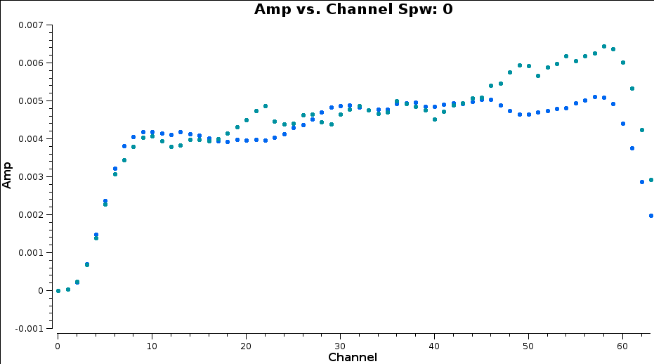
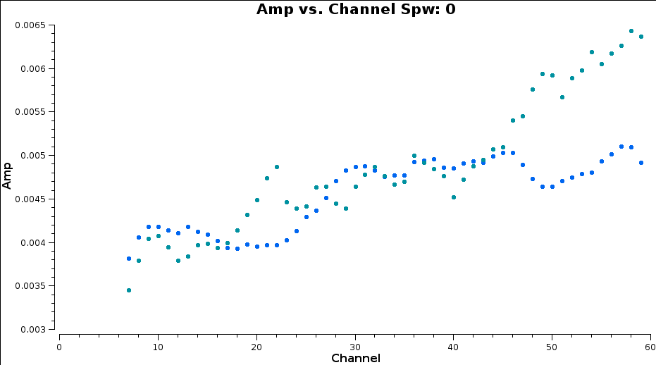
# In CASA:
 default plotcal
 caltable='bpcal.B2';xaxis='freq',
 plotrange=[-1,-1,-180,180]
 iteration='antenna';yaxis='phase';subplot=321
**

# Repeat to plot amplitude
The same wiggles as in B1 (see "Amplitude bandpass solutions B1, coloured by spw") are corrected, but there is a different overall slope (e.g. compare Kn solutions.)
For each calibration source, there is now a flux density and spectral index set for the MS Model column, as well as the delay, phase and improved bandpass calibration. These are used to derive time-dependent amplitude solutions which will both correct for short-term errors and contain an accurate flux scale factor.
Look at the previous time that you ran gaincal, and identify the one thing which you need to change now (apart from the output table name).
# In CASA:
 os.system('rm -rf calsources.ap2')
 default gaincal
 vis='all_avg.ms'
 caltable='calsources.ap2'

**
Plot the solutions
# In CASA:
 default plotcal
 caltable='calsources.ap2'
 xaxis='time';yaxis='amp'
 subplot=321;iteration='antenna';poln='L'
 plotrange=[-1,-1,0.01,0.06]
 plotcal

# Repeat for the other polarization
You expect to see a similar scaling factor for all sources. 1331+305 is somewhat resolved, giving slightly higher values for Cm (the antenna giving the longest baselines).
Finally, we need phase solutions that can be applied to the target source. Because we will interpolate solutions between phase calibrator scans, we just need one phase solution pero phasecal scan. So solint should include all the data from each scan to form a solution.
# In CASA:
 os.system('rm -rf calsources.p2')
 default gaincal
 vis='all_avg.ms'
 caltable='calsources.p2'

**
Plot the solutions
# In CASA:
 default plotcal
 caltable='calsources.p2'
 xaxis='time';yaxis='amp'
 subplot=321;iteration='antenna';poln='L'
 plotrange=[-1,-1,0.01,0.06]
 plotcal

# Repeat for the other polarization
Apply the bandpass correction to all sources. For the other gaintables, for each calibrator (field), the solutions for the same source (gainfield) are applied. Gainfield '' for the bandpass table means apply solutions from all fields in that gaintable. applymode='calflag' will flag data with failed solutions which is OK as we know that these were due to bad data. We use the non-interactive format to allow us to use a loop over all calibration sources.
Cut and paste this all together; press return a few times afterwards till it runs.
# In CASA:
 cals = ['0319+415', '1302+5748', '1331+305', '1407+284']
 for c in cals:
    applycal(vis='all_avg.ms',
             field=c,
             gainfield=[c, '',c,c],
             calwt=F,
             applymode='calflag',
             gaintable=['all_avg.K','bpcal.B2','calsources.p1','calsources.ap2'],
             interp=['linear','nearest,linear','linear','linear'],
             flagbackup=F)                           # Don't back up flags multiple times here
Apply the phase-ref solutions to the target. We assume that the phase reference scans bracket the target scans so linear interpolation is used except for bandpass. Enter the parameters in interactive mode.
# In CASA:
 default applycal
 vis='all_avg.ms'
 field='1252+5634'                                      # This is the target
 gainfield=['**','','**','**']  # Enter the field whose solutions are applied to the target
 calwt=**;
 applymode='**'
 gaintable=['**','**','**','**']
 interp=['**','**,**','**','**']
 flagbackup=True

**
# In CASA:
 default plotms
 vis='all_avg.ms'
 field='1302+5748'                                   # phase-ref
 xaxis='uvdist'; yaxis='amp'; ydatacolumn='corrected'
 avgchannel='64';correlation='LL,RR';coloraxis='spw'

**                 # Note what it looks like and/or make a plotfile and then plot the target.
QUESTION 6 What do the plots of amplitude against uv distance tell you? Answer 6
Split out corrected target data. By default, this will take the corrected column.
# In CASA:
 default split
 vis='all_avg.ms'
 field='1252+5634'
 outputvis='1252+5634.ms'
 keepflags=F
 split
In CASA 4.4 and earlier, you need to correct a minor incompatibility between the e-MERLIN data structure and the expected measurement set format; it does not affect anything except listobs.
# In CASA:
 tb.open('1252+5634.ms',nomodify=F)
 SIDorig=tb.getcol('STATE_ID')
 SID=SIDorig*0
 SIDnew=SID-1
 tb.putcol('STATE_ID',SIDnew)
 tb.close()
WARNING: do not try to run listobs on a Mac, it will not work due to a bug in CASA 4.4 (maybe 4.5)
Instead, click here to see the output you would have got: 1252+5634.listobs.txt
# In CASA:
 default listobs
 vis='1252+5634.ms'
 overwrite=True
 listfile='1252+5634.listobs.txt'

**
Script with all commands to follow the tutorial: 3C277.1_cal_all.py