You should have downloaded and extracted CASA (2015 October: current version 4.4; this tutorial will mostly work in any version from 4.2 on), and the data. See ALMA_IYAS.html for download, file size etc. details and also the credits for the TW Hya data.
The instructions are described in this web page, with some inputs which you have to work out. Please make sure that you understand all task inputs, don't hesitate to ask. There is also a script, twhya.py with the same bits to fill in. You can use its structure as an example to build your own scripts. As a last resort, twhya_withanswers.py is provided.
Make a directory (
tar -xvf sis14_twhya_calibrated_flagged.ms.tar
In the directory with your data, start CASA e.g.
~/CASA/casa-release-4.4.0-el5/casapy
List what is in the Measurement Set visibility data.
# In CASA
default(listobs)                         # Initialise task
inp                                      # View parameters  - do this for any task run interactively
vis='sis14_twhya_calibrated_flagged.ms'  # Set the file name
listobs()                                # Run the task
You can see the task inputs using:
# In CASA
!more listobs.last                    # ! gives access to shell commands
At the end you see:
listobs(vis="sis14_twhya_calibrated_flagged.ms",selectdata=True,spw="",field=""
,antenna="",uvrange="",timerange="",correlation="",scan="",intent="",feed="",arr
ay="",observation="",verbose=True,listfile="",listunfl=False,cachesize=50,overwr
ite=False)
The listobs output first lists scans:
  Date        Timerange (UTC)          Scan  FldId FieldName             nRows     SpwIds   Average Interval(s)    ScanIntent
  19-Nov-2012/07:36:57.0 - 07:39:13.1     4      0 J0522-364                 4200  [0]  [6.05] [CALIBRATE_BANDPASS#ON_SOURCE,CALIBRATE_PHASE#ON_SOURCE,CALIBRATE_WVR#ON_SOURCE]
              07:44:45.2 - 07:47:01.2     7      2 Ceres                     3800  [0]  [6.05] [CALIBRATE_AMPLI#ON_SOURCE,CALIBRATE_PHASE#ON_SOURCE,CALIBRATE_WVR#ON_SOURCE]
              07:52:42.0 - 07:53:47.6    10      3 J1037-295                 1900  [0]  [6.05] [CALIBRATE_PHASE#ON_SOURCE,CALIBRATE_WVR#ON_SOURCE]
              07:56:23.5 - 08:02:11.3    12      5 TW Hya                    8514  [0]  [6.05] [OBSERVE_TARGET#ON_SOURCE]
              08:04:36.3 - 08:05:41.9    14      3 J1037-295                 1900  [0]  [6.05] [CALIBRATE_PHASE#ON_SOURCE,CALIBRATE_WVR#ON_SOURCE]
...
This shows that the individual integration time (after previous averaging) was 6.05 sec and the following sources were used:
| J0522-364, 3c279 | Bandpass calibration |
| CERES | Primary flux calibration |
| J1037-295 | Phase reference source, observed in ~1 min scans, alternately with |
| TW Hya | Target, observed in ~5.5 min scans |
There is just one spectral window 234 MHz wide, (originally in the second baseband, BBC) divided into 384 channels (also pre-averaged), and the first channel is at f = 372.533086 GHz (remember this).
| SpwID | Name | #Chans | Frame | Ch0(MHz) | ChanWid(kHz) | TotBW(kHz) | CtrFreq(MHz) | BBC Num | Corrs |
| 0 | ALMA_RB_07#BB_2#SW-01#FULL_RES | 384 | TOPO | 372533.086 | 610.352 | 234375.0 | 372649.9688 | 2 | XX YY |
Finally, there are 21 antennas present.
Plot the data for some of the sources, amplitude against uv distance (projected baseline length), averaging all channels and 30 sec.
# In CASA
default(plotms)
vis='sis14_twhya_calibrated_flagged.ms'
xaxis='uvdist'
yaxis='amp'
avgchannel='384'
avgtime='30s'
field='Ceres, TW Hya, J1037-295'
coloraxis='field'
plotms
Make a note of the approximate longest baseline length, B. You see that Ceres is very resolved on baselines longer than 250 m. What about TW Hya? (NB colours may differ on various operating systems, you can change this using the Display tab or parameter customsymbol).
There is a very little bad data; for speed we will ignor it for now but see Flagging for a worked example when you have time.
Task clean is used to Fourier transform the visibilities into the image plane (dirty image) and then remove artefacts due to gaps in the uv coverage by subtracting the sidelobes of the dirty beam. You should have noted the observing frequency f from the first listobs, and longest baseline length B in the amplitude v. uv distance plot. Use this to estimate roughly the resolution of the synthesised beam. You can use the Python capability in CASA if you want (note that numbers need to be written with a floating point as in res or else python will interpret them as integers):
# In CASA
B =                             # set variable for longest baseline, in m
f =                             # approx. observing frequency, in Hz
c = 2.998e8
res = 3600.*degrees( (c/f)/B )  # approx. resolution, in arcsec
The image pixel (cell) size should be smaller than 1/3 of the synthesised beam, here we use 1/6. Enter your estimate, i.e. res/6 (rounded to the nearest 0.01 arcsec) as cell below. It should be in the range [0.05, 0.1] arcsec; if not, check your calculations!
In a compact ALMA configuration like this, a small image will cover most of the primary beam. The antenna diameter D is 12 m, so repeat the calculation above with D instead of B to estimate the FWHM. We will set the total image size (imsize) to be about 1.5 *FWHM, in pixels, rounded to the nearest 50. It should be in the range [200, 300].
# In CASA
clearcal('sis14_twhya_calibrated_flagged.ms') # Remove previous self-cal
os.system('rm -rf twhya_cont_clean0*') #   Delete any old images of the same name

default(clean)
vis='sis14_twhya_calibrated_flagged.ms'
imagename='twhya_cont_clean0'
field='TW Hya'
mode='mfs'
cell=['***arcsec']             # Enter pixel size
imsize=[***,***]               # Enter image size in pixels
weighting='natural'
niter=500
interactive=True

inp

clean
Follow the tutorial demonstration of how to set a mask, etc. Note that prior knowledge of TW Hya suggests that the real emission is within a few arcsec of the centre only. Clean will make acertain number of iterations (default 100) and then display the residual image after having subtracted the brightest points and their sidelobes. Continue, exending the mask if necessary, until the source area has no emission brighter than the surrounding noise. In early stages like this is is better to clean less if in doubt; you may want to go deeper after the self-calibration.
Inspect the image. Once the viewer is open, you can use the spanner icon to get a menu to change the contrast etc. and draw a box to measure the off-peak noise. The rms in the box is given in the panel from View - Regions - Statistics (see First continuum image of TW Hya below).
# In CASA
viewer('twhya_cont_clean0.image')
For consistency, it is better to script measuring the S/N. Add the Cursors pane and make a note of the pixel coordinates (bottom left corner, top right corner) of a suitable, large but off-source region, and then of a box enclosing the source and enter them in imstat.
# In CASA
off = '**,**,**,**'  # your off-source box

default(imstat)
imagename='twhya_cont_clean0.image'
box=off       # enter off-source pixel coordinates

imstat
Better still, you can define variables to hold the imstat output. Make a note of the values, to check that self-calibration improves the image.
# In CASA
off = '**,**,**,**'  # your off-source box
on = '**,**,**,**'  # your on-source box

rms1=imstat(imagename='twhya_cont_clean0.image',
     box=off)['rms'][0]    # enter off-source pixel coordinates

peak1=imstat(imagename='twhya_cont_clean0.image',
      box=on)['max'][0]       # enter on-source pixel coordinates

print 'twhya_cont_clean0.image rms %7.3f mJy' % (rms1*1000.)
print 'twhya_cont_clean0.image peak %7.3f mJy/bm' % (peak1*1000.)
print 'twhya_cont_clean0.image S/N %7f mJy/bm' % (peak1/rms1)
I got S/N 30 (65 if the extra flagging is done); if you get very much less, ask for help. Enter the pixel coordinates in twhya.py at the top of the script.
Because the origin of phase is arbitrary, we need to pick an antenna to have its phase corrections chosen to be zero. Plot the locations of the antennas.
# In CASA
default(plotants)
vis='sis14_twhya_calibrated_flagged.ms'
plotants
Choose an antenna close to the centre of the array but not so close to other antennas that it might be shadowed (DA41, DV01, DV04, DV07,DV5, DV17 and DV21 are shadowed or flagged already for other reasons) nor the two which you partly flagged above. If in doubt, see the one marked on this plot.
When you ran clean, the Fourier Transform of the Clean Components was recorded in the Measurement Set as the Model. Plot this just for illustration:
# in CASA
default(plotms)
vis='sis14_twhya_calibrated_flagged.ms'
xaxis='uvdist'
yaxis='amp'
ydatacolumn='model'
avgchannel='384'
avgtime='30s'
field='TW Hya'
coloraxis='baseline'
plotms
You can also plot the data, or data-model, etc. by selecting Data Column interactively (Axis tab). This composite plot shows that the model is a fairly good fit to the data but contains some spurious components on short spacings; you may not have so much if you cleaned more cautiously.
The task gaincal compares the data with the model and uses a chi-sq minimisation to find the corrections for each antenna which will make the data on all baselines resemble the model most closely, for each chosen solution interval. Phase errors have a worse effect so we correct those first. The solution interval (solint) should be such that any systematic errors don't change much but there is enough averaging to provide good S/N per antenna. This is established by examining the phase and estimating the sensitivity - or, as here, for speed, by making an educated guess based on previous ALMA data reduction.
#In CASA
os.system('rm -rf twhya_cont.ph1')         # Remove any old table of the same name

default(gaincal)
inp(gaincal)                               # Look at the options for calmode
vis='sis14_twhya_calibrated_flagged.ms'
caltable='twhya_cont.ph1'
field='TW Hya'
solint='30s'
calmode='**'                               # Phase only
refant='**'                                # Your chosen refant
inp

gaincal
Don't worry about the messages about failing ~10 percent of solutionsin some time slots (but if most of the solutions fail, something is wrong). Plot the solutions. Use the 'next' button to see the rest of the antennas. Although there is some scatter, there are no very wild points (which would suggest bad data) or a systematic curve on many antennas (which would suggest a bad model).
#In CASA
default(plotcal)
caltable='**'              # The table you just made
xaxis='**'                 # Plot phase against time
yaxis='**'
subplot=531
iteration='antenna'
plotrange=[-1,-1,-180,180]
plotcal
Apply the solutions. This will create a CORRECTED column in the measurement set. After applycal has finished, try plotting this in plotms if you have time.
#In CASA
default(applycal)
vis='sis14_twhya_calibrated_flagged.ms'
field='TW Hya'
gaintable=['twhya_cont.ph1']
applycal
Image the phase-self-calibrated data. Most things apart from the output image name is the same as before (unless you want to improve something), so enter all the required parameters and values. However, because we can clean more deeply, the number of iterations is increased.
#In CASA
os.system('rm -rf twhya_cont_clean_p1*') #   Delete any old images of the same name
default(clean)
vis='sis14_twhya_calibrated_flagged.ms'
imagename='twhya_cont_clean_p1'
...                                 # Enter parameters required
niter=1000
npercycle=200
interactive=True
inp

clean
Check the noise in your new image. Use your chosen box sizes. You could also inspect it in the viewer. You will see (or you may have noticed during imaging) that the remaining errors are symmetric, characteristic of amplitude errors. I got a new S/N of nearly 50 (higher if the extra flagging was done), so a big improvement.
#In CASA
# You only need to re-enter these if you have exited and re-started CASA
off = '**,**,**,**'  # your off-source box
on = '**,**,**,**'  # your on-source box

rms1=imstat(imagename='twhya_cont_clean_p1.image',
     box=off)['rms'][0]

peak1=imstat(imagename='twhya_cont_clean_p1.image',
      box=on)['max'][0]

print 'twhya_cont_clean_p1.image rms %7.3f mJy' % (rms1*1000.)
print 'twhya_cont_clean_p1.image peak %7.3f mJy/bm' % (peak1*1000.)
print 'twhya_cont_clean_p1.image S/N %7.f' % (peak1/rms1)
Now we repeat the main self-calibration steps to use our new model in calibrating the amplitude (and any residual phase corrections based on the improved model). gaincal uses the DATA column, so we apply the previous phase-only corrections (gaintable) as well as writing a new caltable. The other parameters as before.
#In CASA
os.system('rm -rf twhya_cont.ap1')
default(gaincal)
vis='sis14_twhya_calibrated_flagged.ms'
caltable='twhya_cont.ap1'    # the new table
...                          # enter parameters needed
calmode='**'                 # amplitude and phase
gaintable='twhya_cont.ph1'   # apply the previous calibration
refant='DV22'
inp

gaincal
Check the solutions. The phase solutions should be smaller and the amplitude solutions scattered around 1, which indeed they are.
#In CASA
default(plotcal)
caltable='twhya_cont.ap1'
xaxis='time'
yaxis='phase'
subplot=531
iteration='antenna'
plotrange=[-1,-1,-180,180]
plotcal

default(plotcal)
caltable='twhya_cont.ap1'
xaxis='time'
yaxis='amp'
subplot=531
iteration='antenna'
plotrange=[-1,-1,0,2],
plotcal
Apply the original phase-only solutions and these phase and amplitude solutions.
#In CASA
default(applycal)
vis='sis14_twhya_calibrated_flagged.ms'
field='TW Hya',
gaintable=['**','**']                       # both calibration tables
inp

applycal
Finally, clean again. In a real situation, you might want to experiment with different (shorter) solution intervals, investigate whether outlier solutions are due to bad data and so on, until either there is no further improvement or you have reached the theoretical noise for the time on source and number of antennas. In this case the expected rms is about 1 mJy and I got to 1.4 mJy, but for these early data probably there is not much more improvement possible. You could also experiment with different weighting in clean, see the CASA guide.
#In CASA
os.system('rm -rf twhya_cont_clean_ap1*') #   Delete any old images of the same name
default(clean)
vis='sis14_twhya_calibrated_flagged.ms',
imagename='twhya_cont_clean_ap1'
...                                        # Enter the parameters
interactive=True
inp

clean
Now run imstat again. I got S/N 369 and a new peak of 528 mJy/beam, which is slightly higher than previously. Be careful that the amplitudes do not change too much, which would suggest an incorrect model. Check the image in the viewer if you have time.
The next stage is to split out the CORRECTED column of target data in order to prepare for line imaging. If your final TW Hya continuum image looked bad and you think that something has gone wrong, you can use a ready-made file instead, you should have twhya_calibrated_flagged.ms.tar already (and also a ready made twhya_cont_clean_ap1.image.tar). If not, get it from a tutor or see download link. If you already have an ms of the same name, delete or move it before you extract twhya_calibrated_flagged.ms from the tarball. Assuming you don't need to use the ready-made file:
#In CASA
os.system('rm -rf twhya_calibrated_flagged.ms')
default(split)
vis='sis14_twhya_calibrated_flagged.ms'
field='TW Hya'
outputvis='twhya_calibrated_flagged.ms'
keepflags=F
inp

split
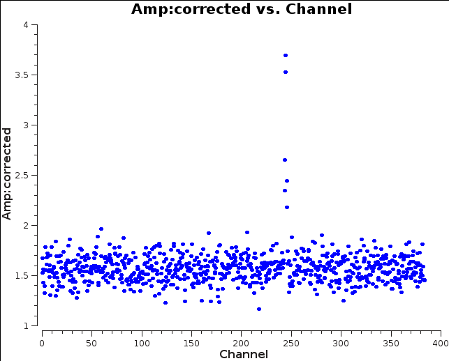
Now look for the line again, using the shorter baselines.
#In CASA
default(plotms)
vis='twhya_calibrated_flagged.ms'
xaxis='channel'
yaxis='amp'
ydatacolumn='data'
uvrange='0~50'
avgtime='1e9'
avgscan=True
avgbaseline=True
plotms
Visibility spectrum of TW Hya
on baselines less than 50 m. Use the magnifying glass icon (bottom left) to zoom in. The line is clearly seen in at least 3 channels. For safely we exclude a larger range of 40 channels approximately centred on the line. Enter this in uvcontsub below, filling in the lower and higher channel limits around the line.
#In CASA
os.system('rm -rf twhya_calibrated_flagged.ms.contsub')
default uvcontsub
vis = 'twhya_calibrated_flagged.ms'
field = 'TW Hya'
fitspw = '0:**~**'   # Two integers defining the channel range around the line
excludechans = True
fitorder = 1
solint='int'

uvcontsub
You can inspect the output twhya_calibrated_flagged.ms.contsub in plotms if you have time.
In this case, there was existing knowledge that the line peak is at about 3 km/s Vlsr, so we use clean in velocity mode. From listobs, the channel width is 610.352 kHz and the NH2+ rest frequency is 372.67249 GHz, giving a spectral resolution of ~0.5 km/s. This time, we try a different (more uniform) weighting, which will give a smaller synthesized beam at the expense of slightly higher noise.
#In CASA
os.system('rm -rf twhya_n2hp.*')
default(clean)
vis = 'twhya_calibrated_flagged.ms.contsub'
imagename = 'twhya_n2hp'
field = 'TW Hya'
mode = 'velocity'
nchan = 15
start = '0.0km/s'
width = '0.5km/s'
outframe = 'LSRK'
restfreq = '372.67249GHz'
interactive = T
imsize = [250, 250]
cell = '0.08arcsec'
weighting = 'briggs'
robust = 0.5
inp

clean
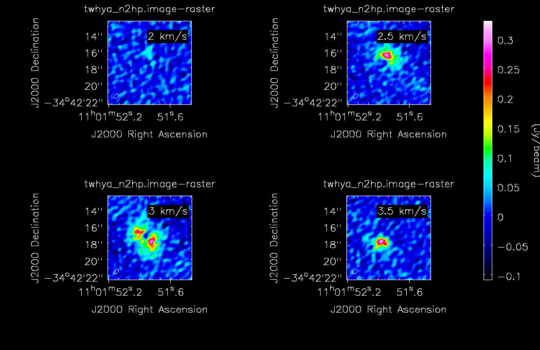
Look at the interactive clean tool options. Make sure that you have View Animator enabled and play though the channels until you see the emission. You can either set a separate mask for each channel with emission, or click the button to apply one mask to all channels. Either will do here; if there are many channels with emission then the second approach is easier and usually OK for ALMA's good uv coverage.
Inspect twhya_n2hp.image in the Viewer. The channels with emission should look something like:
Central channels with NH2+ emission
. You can explore the other viewer image analysis tools. You will see that there is an N-S velocity gradient.
There are also scriptable tasks to perform many of these analyses, for example making a moment image. Measure the off-source rms in the image as a lower bound. Check the channel range with emission and add a few channels each side.
#In CASA
os.system('rm -rf twhya_n2hp.mom0')
immoments(imagename='twhya_n2hp.image',
outfile='twhya_n2hp.mom0',
includepix=[**,**],               # Set values to the off-source rms and much greater than peak
chans='**~**',                    # Choose about 9 channels round the peak
moments=[0])
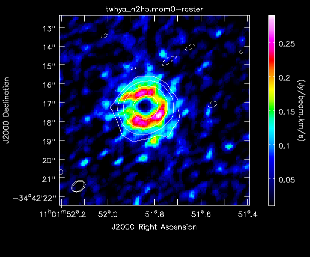
You can load the moment map in the viewer and overlay continuum contours, or here is a scriptable recipe (see help imview for details); in twhya.py it will write a plotfile instead of the viewer.
#In CASA
imview(raster={'file': 'twhya_n2hp.mom0',
               'colorwedge': T},
       contour={'file': 'twhya_cont_clean_ap1.image',
                'unit': 0.004,
                'levels': [-1,1,4,16,64] },
       zoom=2)
Zeroth moment overlaid with continuum contours
Finally, if you want to do more analysis outside CASA, you can export images as FITS, here is an example.
    exportfits(imagename='twhya_n2hp.image',
               fitsimage='twhya_n2hp.image.fits')
amsr@jb.man.ac.uk 15 Oct 2015